Stokes Drag (free fall + linear air drag force)

­ ­ ­­Let us study a somewhat more complex case of motion in a gravitational field. Instead of just the force of gravity, let us add a drag force which is proportional to the velocity, that is:

$${\bf F} = - \alpha {\bf v}.$$

In other words, at every instant, the drag force is proportional to the velocity and has­ an opposite direction. The constant of proportionality­ α includes all the physics of the flow around the object, and for us, it is simply assumed to be given.

Just for general knowledge, such a drag law does exist. It describes the drag on objects moving in a very viscous fluid, such as a marble droped through ho­ney. In such a case, the parameter α will depend on the size of the marble and the viscosity of the honey (the actual dependence is beyond the scope of this course, if you’re curious though, it is linear in the radius and the viscosity, as is explained here). In less viscous cases, such as a marble dropped through air, the drag force typically grows like the velocity to a higher power (usually close to 2). But this we will leave for the example below!

Back to our problem. If the only forces are that of gravity and drag, the second law of motion would imply that:

$$m {d{\bf v} \over dt} = {\bf F}_g + {\bf F}_d = m {\bf g} - \alpha {\bf v}$$

How does this equation behave?

To answer this question, we will try to understand the behavior before we actually solve the equation.

First, in the limit of small velocities, we find that the drag which of course is proportional to the velocity, is small as well, and can therefore be neglected. Once this is done, we find the trivial case of free fall:

$$\require{cancel} m {d{\bf v} \over dt} = {\bf F}_g + \cancelto{0}{{\bf {F}}_d} \approx m {\bf g} ~~\Rightarrow~~v\approx g t$$

(again, we define the positive direction to be down, hence the velocity increases).

For large velocities, we expect the acceleration term to dissapear, giving a balanced gravitational and drag forces, from which we can derive the asymptotic velocity:

$$\require{cancel} \cancelto{0} {m {d{\bf {v}} \over dt}} \approx {\bf F}_g + {\bf F}_d = m {\bf g} - \alpha{\bf v} ~~\Rightarrow~~v_{\infty} = {m g \over \alpha}.$$

From the two limiting behaviors, we can draw a heuristic graph, as can be seen in the figure.

Now that we understand the behavior of the falling object, we can solve for the actual motion. If we take the z component of eq. (1) above (i.e., take the scalar product $\cdot {\hat{\bf z}}$ on both sides, we get the scalar equation:

$$m { dv_z \over dt} = m g - \alpha v_z .$$

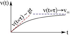
The velocity as a function of time. For small t’s, the velocity is small, the drag is therefore negligible and the motion is that of free fall. Hence, v grows linearly. For large t’s, the velocity approaches its asymptotic value, where the drag equals gravity.

This equation is a differential equation because it relates a variable, v_z, to its derivatives (in this case, to its first derivative dv_z/dt). How do we solve such an equation? Well, the truth is that solving differential equations is an art. There is no recipe to solve all differential equations just as there is no recipe to solve all integrals. Each differential equation, just like every integral, requires knowing how to solve that particular type, or how to transform it to a form for which a solution is known.

This type of equation can be solved through separation of variables. See inset below for how they are generally solved. It is one of two types of equations which we will solve in this course.

In our case, we separate the t’s and dt’s to one side, and the v_z’s and dv_z’s to the other side. We obtain:

$$m { dv_z \over m g - \alpha v_z} = dt .$$

What this equation implies is that for any infinitesimally small time step dt, there will be the same change in the velocity dv_z times the paritular function of v_z. To get the actual v_z(t), we will have to integrate over many of those changes, over time on one hand, and over dv_z on the other. We omit the “z” for brievety:

$$\int_{v=0}^{v(t)} {m dv \over m g - \alpha v} = \int_{t=t_0}^{t} dt .$$

Note:

In this course, we will learn to solve two types of differential equations, those which can be solved through separation of variables, and linear equations, which will pop-up once we solve oscillatory motion. So how do we solve seperable differential equations? Well, as the name suggests, we can separate the variable from the unknown function,

Example 1: Terminal Velocity for high velocity drag

In the high velocity limit, the drag force on a body can be shown to depend on the air density $\rho$ and the total cross-section of the body, $A$ as follows

$${\bf F}_d = - {1 \over 2} C_d \rho v^2 A {\bf \hat v},$$

where $C_d$ is the drag coefficient (the factor 1/2 is there for convention). It depends on the geometry of the body (for example, a smooth sphere typically has $C_d \sim 0.1$).

Q. Given that this is the drag at high velocities (when the flow around the body is turbulent), what is the terminal velocity of a free falling object?

A. The terminal velocity is the asymptotic velocity of the object, namely, at this velocity there is no more acceleration and the net forces therefore have to vanish. Thus,

$$m \cancelto{0}{{d{\bf v} \over dt}} = m{\bf g} - {\bf F}_d = -m g {\hat {\bf z}} - {1\over 2} \rho v^2 C_d A {\bf \hat{v}}.$$

If we consider the ${\hat \bf z}$ component, we have

$$mg = {1\over 2 } C_d A \rho v_z^2$$

or,

$$v_z = \sqrt{2 m g \over C_d A \rho} .$$

This is the terminal velocity.

Example 2: Free fall motion with high velocity drag

Q: What is the velocity v(t) of an object falling from rest in the high velocity limit?

A: The equation of motion is given by

$$m{d{\bf v} \over dt} = m{\bf g} - F_d = -m g {\hat {\bf z}} - {1\over 2} \rho v^2 C_d A {\bf \hat{v}}.$$

If we take the z-direction component, and define it to be pointing down(!) then

$$m{d v_z \over dt} = m g - {1\over 2} C_d A \rho v_z^2 .$$

This differential equation can be separated, we find (after ommiting the z index):

$$m{d v \over m g - {1\over 2} C_d A \rho v^2 } = dt ,$$

and integrated over:

$$\int_{v=0}^{v} m{d v_z \over m g - {1\over 2} C_d A \rho v^2 } = \int_{t=0}^t dt .$$

We begin from v=0 since the object starts from rest. We find:

$$\sqrt{2 m \over A C_d g \rho} \tanh^{-1} \left( \sqrt{A C_d \rho \over 2 g m} v \right)= t .$$

Or inverting it:

$$v(t) = \sqrt{2 g m \over A C_d \rho} \tanh \left( \sqrt{A C_d g \rho \over 2 m} t \right) .$$

Written more nicely, we have

$$v(t) = v_\infty \tanh \left( t / \tau \right)$$

with

$$v_\infty = \sqrt{2 g m \over A C_d \rho}, ~~~~\tau = v_\infty/g .$$