Modeling the COVID-19 / Coronavirus pandemic – 4.Modeling with at time variable infection rate.

A more realistic assumption than the approximation above is to allow the infection rate to be time dependent. This time dependency was derived in the first post, by using the results of Cereda et al. 2020 who used a $\Gamma$-distribution to fit the interval between the appearance of symptoms in infectors and infectees. After removing the widening by the incubation period, we derived the serial interval of infections, which is the normalized infection probability, namely

$$\beta(t) = R_0 {b^a t^{a-1} \exp(-b t) \over \Gamma(a)},$$

with $a = 3.1 \pm 0.8$ and $b = 0.47 \pm 0.12$ days$^{-1}$.

Given this infection rate, can we derive the relation between the exponential growth rate $r$ and the basic reproduction number $R_0 = \int_0^\infty \beta(t) dt$? Can we predict by how much the growth will slow down if we quarantine at a given rate, or decrease the infection rate (e.g., through social distancing)?

To get the $r$, we assume that the number infected at a given time is $I = I_0 \exp(rt)$. This means that the rate at which people are infected is its derivative $\dot{I} \equiv dI/dt = r I_0 \exp(rt)$. The basic equation for the infection rate is the following. At each instant $t$, there are people who were infected at a previous time $t-\tau$ who now infect at a rate $\beta(\tau)$. We therefore have the equation

$$\dot{I}(t) = \int_{0}^\infty \beta(\tau) \dot{I}(t-\tau) d\tau .$$

We now insert our “guess” which is the exponential growth and find that

$$r I_0 \exp(rt) = \int_{0}^\infty \beta(\tau) r I_0 \exp\left(r(t-\tau)\right) d\tau ,$$

which after cancellation of $r I_0\exp(rt)$ gives

$$1 = \int_{0}^\infty \beta(\tau) \exp \left( -r \tau \right) d\tau .$$

This is the basic equation relating the growth rate $r$ to the infection rate function $\beta(t)$, which itself depends on the basic reproduction number $R_0$.

For the $\Gamma$ distribution given above, the equation becomes:

$${1\over R_0} = \int_{0}^\infty {b^a \tau^{a-1} \exp\left(-(b+r) \tau \right) \over \Gamma(a)} d\tau = {b^{a} \over (b+r)^a}.$$

With the above values of $a$ and $b$, this implies that the basic reproduction number is high and equal to $R_0 = 4.6 \pm 2.7$.

If we take the growth observed in Japan, we find $R_{0,J} = 1.6 \pm 0.3$.

Since the errors on $R_0$ and $R_{0,J}$ are correlated, it is also worth while looking directly at the ratio:

$${R_{0,J} \over R_0} = \left(b+r_{0,J} \over b+r_0\right)^a = 0.34 \pm 0.15$$

Namely, the Japanese social norms implies that they are about 3 times less infectious than typical societies.

The effect of quarantining and “social distancing” can also be included in the calculation by modifying the infection rate. For example, suppose that there is a quarantining rate $\kappa$, and that we reduce the reproduction number to a fraction $\epsilon$, namely that $R = \epsilon R_0$. We then get a modified infection rate of

$$\beta_\mathrm{mod}(t) = \epsilon R_0 {b^a t^{a-1} \exp \left(-b t\right) \over \Gamma(a)} \exp(-\kappa t).$$
Since a $\Gamma$-distribution times an exponent is another (but not normalized) $\Gamma$-distribution, we can easily integrate and find that

$${1\over \epsilon R_0} = {b^{a} \over (b+r +\kappa)^a}.$$

The solution is

$$r = b \left[ (\epsilon R_0)^{1/a} -1\right] -\kappa = (r_0 + b) \epsilon^{1/a} - b - \kappa.$$

For the second equality we plugged in the solution for $R_0$ from the observed $r_0$ - the growth under natural conditions.

Clearly, for no social distancing ($\epsilon=1$), we need $\kappa$ as fast as the $r_0$ of the base case (without any social modifications). Namely, we need to quarantine people as fast as $1/r_0 = 3.3 \pm 0.7$ days. A place like Iran or Bnei Brak requires quarantining as fast as $2.25 \pm 0.25$ days from the day of infection, while Japan or Sweden, more like $13.5 \pm 5$ days.

We can look at it differently. Without quarantining we need to reduce the social interactions to a fraction $\epsilon = (b/(r_0+b)^a = 1/R_0$, which is the above result.

In fig. 1 we plot the growth rate as a function of the quarantining time $1/\kappa$ and social distancing factor $1/\epsilon$.

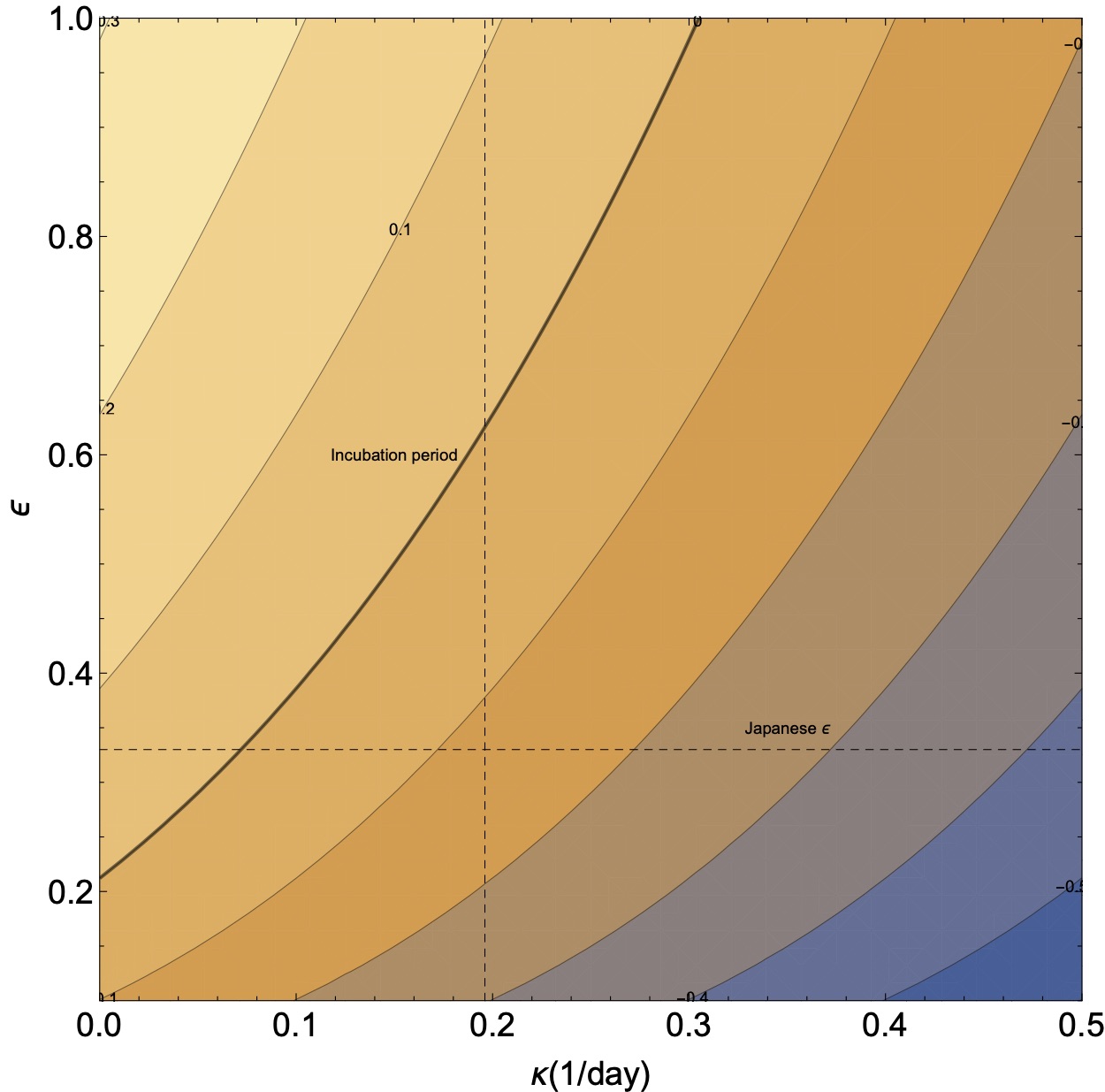
Figure 1 - The value of $r$ as a function of the quarantining rate $\kappa$ and the social distancing $\epsilon$. The top left corresponds to normal conditions. The dashed lines corresponds to the values that can reasonably be expected if societies behave as the Japanese, or if we quarantine as fast as the incubation period.

 

One apparent conclusion is that under normal conditions (i.e., for $R=R_0$), asking anyone who has any coronavirus like symptoms to quarantine himself is insufficient to stop outbreaks. This is because the typical incubation period is 5 days, which is larger than the necessary quarantining time. The exception might be a society like Japan in which the quarantining time is longer than the incubation time. However, this is still without having taken the asymptomatic coronavirus carriers.

Effect of asymptomatic carriers

If we have asymptomatic carriers, then we will not be able to detect and quarantine them (unless they are discovered by a more sophisticated protocol, such as checking all those who were in contact with a sick person). This means that the quarantining fraction does not decay as $\exp(-\kappa t)$ but as $f + (1-f) \exp(-\kappa t)$. Once we plug this factor to $\beta_\mathrm{mod}(t)$ and integrate over, we obtain

$${1\over \epsilon R_0} = f {b^{a} \over (b+r)^a} + (1-f){b^{a} \over (b+r +\kappa)^a}.$$

This equation does not have an analytical solution for $r$. We can however solve for $r=0$, and find the quarantining rate necessary to stop the outbreak. It is

$$\begin{aligned} \kappa_\mathrm{crit} &=& \left[\left(\frac{(1-f) R_0 \epsilon }{1-f R_0 \epsilon }\right)^{{1}/{a}}-1\right] b \\ & = & \left[\left(\frac{(1-f) \epsilon (b+r_0)^a}{b^a - f \epsilon (b+r_0)^a}\right)^{{1}/{a}}-1\right] b. \end{aligned}$$

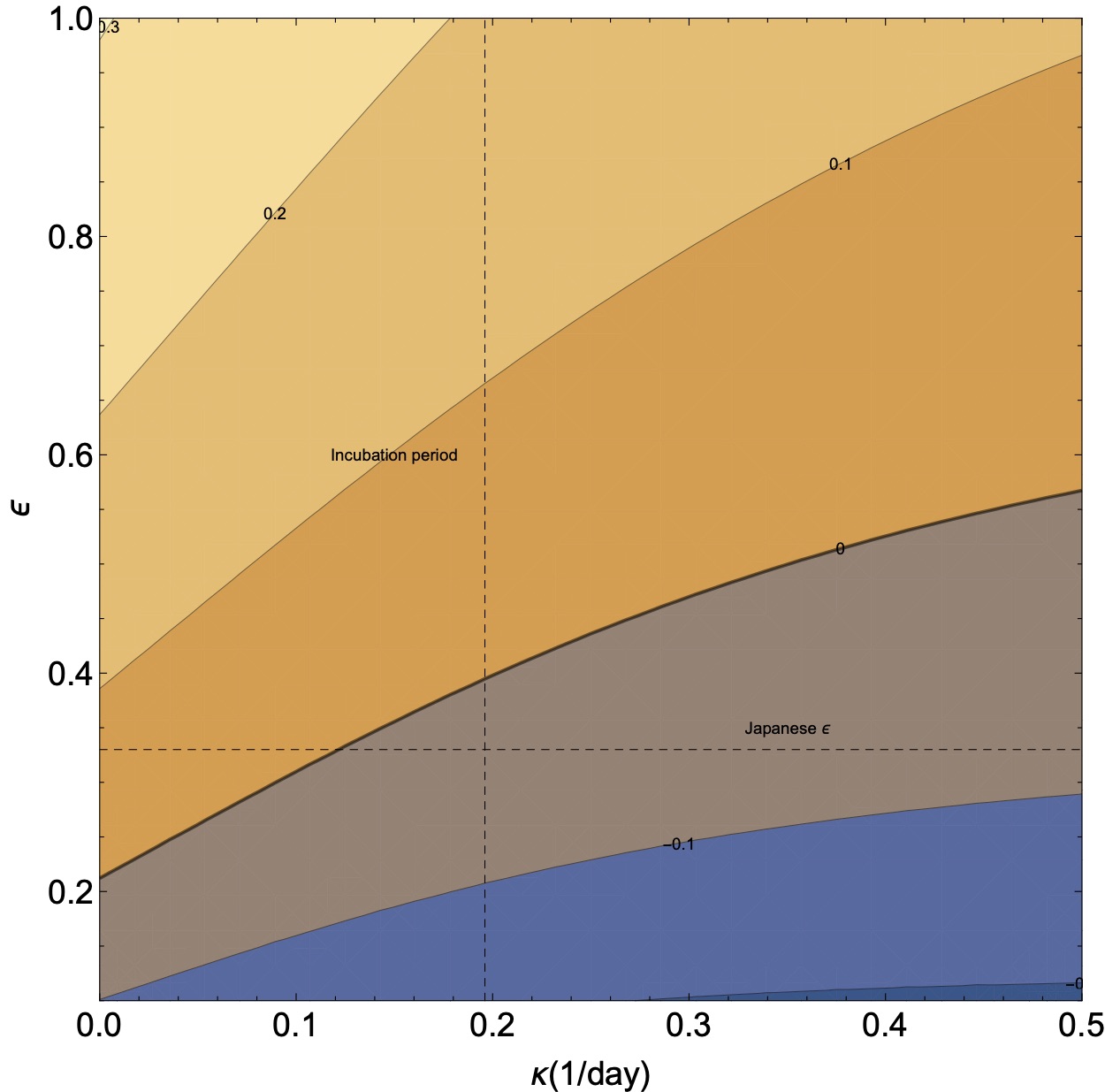
Figure 2 - The same as fig. 1, with the inclusion of asymptomatic patients that are not quarantined.

 

In fig. 2 we plot the rate $r$ as a function of the quarantining and social distancing. For our canonical value of the asymptomatic infected, we find that there is no $\kappa$ that will give $r=0$. Namely, the growth just from the asymptomatic is sufficient to cause an epidemic if the social interaction stays the same. If we use the rate observed in Japan, $r_J$, we find that $\kappa_\mathrm{crit} = 0.13 \pm 0.06$, which gives a typical critical time of 8 days to quarantine.

Let us now switch gears and simulate the pandemic numerically. This will allow us to easily incorporate more complex scenarios, such as different conditions for quarantining.

Additional posts in the series include

1. Background data
2. Simple Modeling
3. Effects of several populations with a variable infection rate
4. Modeling with at time variable infection rate (this page)
5. Numerical Model (coming soon!)
6. Discussion and Conclusions (coming soon!)