The Foucault Pendulum

Background

Foucault’s Pendulum, (the Panthéon, Paris, Photograph taken by Michael Reeve, 30/1/04)

The Foucault Pendulum was conceived by Léon Foucault in the middle of the 19^th century, with the goal of proving Earth’s rotation through the effect of the Coriolis Force. In essence, the Foucault Pendulum is a Pendulum with a long enough damping rate such that the precession of its plane of oscillations can be observed after typically an hour or more. A whole revolution of the plane of oscillation takes anywhere between a day if it is at the pole, or longer at lower latitudes. At the equator the plane of oscillation does not rotate at all. (Note that if a precession period is defined as a rotation of 180° of the plane of oscillation, then the period at the pole is 12 hrs).

Other effects which were used to demonstrate the rotation of the Earth include:
• The aberration of starlight. The effect, which is akin to the Doppler effect implies that light arriving from a moving source (or to a moving observer) arrives at different angles. This effect is similar to the changing apparent motion of rain drops while walking at different speed. Because earth is moving relative to the stars, there is an annual aberration, while because of Earth’s daily rotation, there is a small but measurable diurnal aberration.
• Earth’s flattening. Because of Earth’s rotation, the centrifugal forces imply that a mass at the equator is more weakly pulled towards the center of Earth than a mass at the pole. The result, Earth has the shape of an oblate sphere. The equatorial and polar radii are different in one part in 300.

More on Foucault and his Pendulum in Wikipedia.

The Coriolis force responsible for the the pendulum’s precession is not a force per se. Instead, it is a fictitious force which arises when we solve physics problems in non-inertial frames of reference, i.e., in coordinate systems which accelerate such that the law of inertia (dp/dt = F) is not valid anymore. In rotating systems, the two fictitious forces that arise are the centrifugal and Coriolis forces. The centrifugal cannot be used locally to demonstrate the rotation of the Earth because the “vertical” in every location is defined as the combined gravity and centrifugal forces. Thus, if we wish to demonstrate dynamically that Earth’s is rotating, we should consider the Coriolis effect.

Here, we solve the precession of the plane of oscillation of a pendulum. We do so under the following approximations:

(1) The precession rate of the plane of oscillation is slow compared with the oscillation of the pendulum.

(2) The pendulum oscillates with a small amplitude, such that its motion can be approximated as harmonic (a spring).

The derivation involves mapping the pendulum problem into the mass-on-spring problem in two dimensions, and then solving it in polar coordinates, to obtain the equation describing the precession of the oscillation plane.

Pendula as 2D springs systems

The equation of motion of a mathematical pendulum without Coriolis can be written as: $${d L \over d t} = m \ell^2 \ddot{\vartheta} = N_{\mathrm {grav}}$$

where $L$ is the angular momentum relative to the oscillation axis and $N_{\rm grav} = - m g \ell \sin \theta$ is the force moment. We can work here for the moment with scalars because without Coriolis, the motion of the pendulum is in a plane.

We now perform our first approximation. We assume small angle oscillations. That is, we assume that $\sin \vartheta \approx \vartheta$. We find:

$$m \ell \ddot{\vartheta} = - m g \vartheta.$$

Instead of $\vartheta$, we can change our variable from $\vartheta$ to $r = \ell \vartheta$ which is the distance from the axis (under the small angle limit. We find:

$$m \ddot{r} = -{m g \over \ell} r .$$

In other words, the equations describing the pendulum are equivalent (at the small angle limit) to the motion of a spring, with a spring constant given by $k_{\rm eff} = mg/\ell$ and indeed the oscillation frequency of the pendulum is $\omega = \sqrt{k_{\rm eff}/m } = \sqrt{g/l}$ as it should.

We are therefore allowed to describe the pendulum as a mass on spring. In general, the plane of the oscillation can have precession, we therefore write the motion of the pendulum as a 2D mass on spring problem:

$$m \ddot{\bf r} = -k_{\rm eff} {\bf r}.$$

(Without any additional forces, the direction of ${ \bf r}$ remains fixed, but with any non-radial force, such as of Coriolis, it will change).

Adding the Coriolis Effect

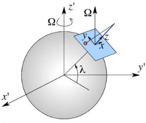
The Rotating coordinate system {x,y,z} is non-inertial since Earth is rotating. As a result, a Coriolis force is added when working in this frame of reference.

We now add the Coriolis force. Since the mass cannot exit the plane, the equation is valid on to the horizontal directions:

$$\displaystyle m \ddot{\bf r} = - {m g \over \ell}{\bf r} - 2 m {\bf \Omega} \times \dot{\bf r}.$$

For convenience, we will work with polar coordinates - $r$ and $\theta$. (Note that this angle $\theta$ is different from the oscillation angle $\vartheta$). The vector ${\bf r}$ and its time derivatives in is polar coordinates, are given by:

$$\displaystyle {\bf r} = r \hat{\bf r}, \quad \dot{\bf r} = {d r \over d t} \rhat + r {d \rhat \over d t} = \dot{r} \rhat + r \dot{\theta}\thetahat$$ $$\displaystyle \ddot{\bf r} = \ddot{r} \rhat + \dot{r} {d \rhat \over d t} + \dot{r} \dot{\theta}\thetahat+ r \ddot{\theta} \thetahat+ r \dot{\theta}{d \thetahat \over d t}$$ $$\displaystyle = (\ddot{ r}-r\dot{\theta}^2)\rhat + (2 \dot{r} \dot{\theta}+ r\ddot\theta) \thetahat.$$

Next, we need to write the Earth’s rotation vector ${\bmOmega}$ in the polar coordinates we use:

$$\displaystyle \bmOmega =\Omega \sin \lambda \hat{\bf z} + \Omega \cos \lambda \cos \theta \rhat - \Omega \cos \lambda \sin \theta \thetahat.$$

Note that the last term is with a minus sign, because $\bmOmega$ has a component opposite to the direction to which $\theta$ grows.

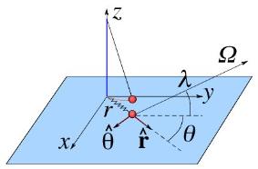
The pendulum and the equivalent spring system in polar coordinates. Once the problem becomes 2D, the oscillations are described by r and θ.

We are now in a position where we can take the ${\thetahat}$ component of the equation of motion. It will gives us the dynamics of the oscillating plane, i.e., how its direction evolves with time. The component is:

$$\displaystyle m r \ddot \theta + 2 \dot{r}\dot{\theta} = - 2 m\left(\Omegabold \times \dot{\bf r} \right)_\theta$$

where the last parenthesis implies that we take the ${\thetahat}$ component of the vector product. Note that $\{ \thetahat , \rhat, \hat{\bf z} \}$ is a right handed system (as can be seen in the figure above). Therefore, the ${\thetahat}$ mcomponent of the product is:

$$\displaystyle \left( {\Omegabold} \times \dot{\bf r} \right)_\theta =\Omega_r \dot{r}_z - \Omega_z \dot{r}_r = -\Omega \dot{r} \sin \lambda,$$

after plugging in the expressions for $\dot{r}$ and ${\Omegabold}$. The equation of motion we find is:

$$\displaystyle m r \ddot{\theta} + 2 \dot{r}\dot{\theta} = 2 m\dot{r} \Omega \sin\lambda.$$

In general, this equation cannot be solved without knowing the time dependence of $r$. However, luckily for us, this equation can be simplified in the limit where the precession is much slower than the oscillations of the pendulum.

The Slow Precession Approximation

If the angular frequency of the pendulum’s oscillations is $\omega$ then we typically have that $\phantom{\int}\dot{r} \sim \omega r\phantom{\int}$. On the other hand, the evolution of the direction of oscillations is given by $\theta$, we expect these variations to be of order a day, the time it takes Earth to complete a revolution, i.e., $\dot{\theta} \sim \Omega \theta$ and $\ddot{\theta} \sim \Omega^2 \theta$ (note that at the end, we have to verify that our solution is consistent with this assumption!).

Since $\phantom{\int}\omega \gg \Omega\phantom{\int}$ then $\ddot{\theta} r$ is smaller than $\dot{r}\dot{\theta}$ by a factor of $\omega/\Omega$ (e.g., if the pendulum has a few sec period, and $2\pi/\Omega$ is of order a day, we are talking about a very small correction, one of 1/10000 that we are neglecting.)

Under this limit, the $r \ddot{\theta}$ term is neglected, and the equation we find is (after canceling out $2 m\dot{r}$):

$$\displaystyle \dot{\theta} = \Omega \sin \lambda.$$

This solution satisfies that $\dot{\theta} \sim \Omega \theta$, thus, our assumption is valid.

The time it takes the pendulum to rotate by $\pi$ radians (i.e., 180°), after which the pendulum appears to have returned to its original state, is:

$$\displaystyle T_{\rm prec} = {\pi \over \dot{\theta}} = {2 \pi \over \Omega} {1 \over 2 \sin \lambda} = {day \over 2 \sin \lambda} .$$

In Jerusalem, for example $\lambda \approx 32^\circ$, it is just under a day. In Paris, it will be shorter.