
On Climate Sensitivity and why it is probably small
What is climate sensitivity?
The equilibrium climate sensitivity refers to the equilibrium change in average global surface air temperature following a unit change in the radiative forcing. This sensitivity, denoted here as λ, therefore has units of °K / (W/m2).(Note that occasionally, the sensitivity, λ is defined as the inverse of the above definition, that is, the radiative forcing required to change the temperature by one degree. This definition is used in the Cess et al. figure below. When in doubt, look at the units!)
Instead of the above definition of λ, the global climate sensitivity can also be expressed as the temperature change ΔTx2, following a doubling of the atmospheric CO2 content. Such an increase is equivalent to a radiative forcing of 3.8 W/m2. Hence, ΔTx2=3.8 W/m2 λ.
The actual value of the climate sensitivity is a trillion dollar question (the cost of implementing Kyoto-like measures). If it is high, it would imply that anthropogenic greenhouse gases could significantly offset the global equilibrium temperature, while if it is small, the anthropogenic effect cannot be large, and any measures we take will not have a noticeable effect. Hence, its value is very important.
The IPCC states (in fact, a dozen times in their third scientific report) that the climate sensitivity is likely to be in the range of ΔTx2 = 1.5 to 4.5°K. Below, we'll try to understand where this number comes from, why it is uncertain (at least for IPCC climatologists who rely on global circulation models) and what we can do about it.
The sensitivity of a Black Body Earth
Let us try to estimate the sensitivity of a Black Body Earth. That is, suppose Earth would have been a perfect absorber of visible and infrared radiation (and therefore also a perfect emitter of those wavelengths). What would its temperature be?In equilibrium, each unit area facing the sun receives a total radiative flux of $$ F_0 \approx 1366 W/m^2 .$$ Thus, the total radiation absorbed by Earth is $$ P_{in} =\pi R^2 F_0,$$ which is the flux times the cross-section of the surface pointing to the sun. The total radiated flux is: $$ P_{out} = 4 \pi R^2 \sigma T^4 ,$$ which is the total surface area of Earth times the flux emitted per unit surface area. σ is the Stephan-Boltzmann constant. In equilibrium, the total absorbed flux equals the radiation emitted, hence, $$ P_{out} = P_{in} ~~\Rightarrow ~~ T = \left(F_0 / 4 \over \sigma\right)^{1/4} = \left(S \over \sigma\right)^{1/4} ,$$ where S = F0/4 is the average flux received by a unit surface area on Earth.
We can now obtain the climate sensitivity, if we differentiate the black body equilibrium temperature of Earth: $$ \lambda = {dT \over dS} = {1 \over 4} {T \over S} = 0.21^\circ K/(W/m^2) .$$ This is the temperature change that would follow a unit change in the radiative flux reaching a unit area on Earth, on average.
The sensitivity of a Gray-Body Earth
In reality, Earth is not a perfect absorber, nor is it a perfect emitter.Because its albedo is not zero, part of the solar radiation is reflected back to space without participating in the radiative equilibrium. Thus, the energy flux absorbed is: $$ P_{in} = \pi R^2 (1-\alpha) F_0,$$ where $\alpha$ is the albedo.
Moreover, because Earth is not a perfect black body, it is not a perfect emitter. Its emissivity ε is less than unity, and the total energy output is: $$ P_{out} = 4 \pi R^2 \epsilon \sigma T^4. $$ The equilibrium now gives:
- This is the often quoted "Black-Body" sensitivity, whereas in fact it is the sensitivity obtained for a Gray Earth, namely, after the albedo is taken into consideration.
- This sensitivity implicitly assumes that by changing the global temperature we don't change the albedo nor the emissivity (aka, no "feedbacks"). We assumed so because when we carried out the differentiation, we didn't differentiate $(1-\alpha)$ nor $\epsilon$.
- This sensitivity translates to an equilibrium CO2 doubling temperature of about 1.2°K.
The effect of feedbacks
The climate system is more complicated than a black body, or a gray body for that matter. In reality, changing the temperature would necessarily change the albedo and also the emissivity.For example, suppose we impose a positive radiative forcing (e.g., we double the atmospheric CO2 content). As a result, the global temperature will increase. A higher global temperature would then imply that there is more water vapor in the atmosphere. However, water vapor is an excellent greenhouse gas, so we would indirectly be forcing more positive forcing which would tend to further increase the temperature (i.e., "a positive feedback").
Next, the higher water content would imply that more clouds are formed. Clouds have two effects, that of a blanket (i.e., reducing the emissivity) and hence increasing the temperature (i.e., more positive feedback). But clouds are white, and thus increase the reflectivity of Earth (increase the albedo). This of course tends to reduce the temperature (i.e., a negative feedback).
Other feedbacks include those of ice/albedo, dust, lapse rate, and even different feedbacks through the ecological system (e.g., see the Daisy World for a nice theoretical example).
Because such feedbacks exist, climate sensitivity is more complicated. Because climate variables (such as the amount of water vapor) should depend on the temperature as the basic variable and not the radiative flux, let us look at the inverse of the sensitivity, and how it depends on temperature. If we differentiate the definition of sensitivity, we find: $$ \lambda^{-1} = {dS \over dT} = {\partial S \over \partial T} + {\partial S \over \partial \alpha} {d\alpha \over dT} + {\partial S \over \partial \epsilon} {d\epsilon \over dT}. $$ Namely, the change in the radiative flux is the direct change associated with a change in temperature (while keeping the albedo and emissivity constant), plus the changes associated with the changed albedo and a changed emissivity. Plugging in eq. (1), we have: $$ \lambda^{-1} = {1 \over 4}{T \over S} + { S \over (1- \alpha)} {d\alpha \over dT} + {S \over \epsilon} {d\epsilon \over dT} $$ Thus, if we wish to estimate the sensitivity of the global climate, we need to know how much the albedo changes if we change the temperature (contributing to $d\alpha / dT$) and how much the emissivity changes as a function of temperature.
For example, more water vapor at higher temperatures implies that the emissivity decreases with temperature (water vapor blocks infrared from escaping), so $d\epsilon /dT$ is negative. This implies that $\lambda^{-1}$ decreases and the sensitivity $\lambda$ increases.
If there are several feedback mechanisms, we can write that each one contributes to a changed sensitivity (both through albedo and through a changed emissivity):
$$ \lambda^{-1} = {dS \over dT} = {\partial S \over \partial T} + \sum_i {dQ_i \over d T} $$
where $dQ_i$ is the effective change to the energy budget through feedback i, following a change in temperature $dT$. The sensitivity can be obtained through two conceptually different methods: Using computer simulations (i.e., global circulation models) and empirically.
Climate Sensitivity from Global Circulation Models
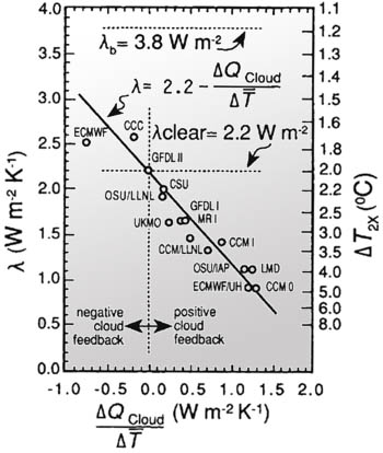
Figure 1 - Results from Cess et al. (1989), showing that the largest contribution to GCM climate sensitivity uncertainty is the cloud feedback. The latter can be characterized by ΔQcloud/ΔT, the cloud related heat change associated with a unit change in temperature. Clearly, cloud feedback is the dominant factor determining climate sensitivity, and the large uncertainty in its value from model to model, implies that different GCMs give wildly different climate sensitivities.
Global circulation models are very powerful tools. Because in principle all the different aspects of the simulations can be controlled and studied, they can serve as detailed "climate laboratories", and thus have notable advantages. Specifically,
- GCMs can be used to analyze the effect of different components in the climate system. For example, one can separate the behavior of different feedbacks (e.g., water vapor, ice, etc.).
- GCMs can be used to estimate the effects of different types of forcing. This is because different geographic distribution of forcings can in principle cause different regional variations and in principle even different global temperature variations (even if the net change to the radiative budget is the same!)
The above figure explains why this large uncertainty exists. Plotted are the sensitivities obtained in different GCMs (in 1989, but the situations today is very similar), as a function of the contribution of the changed cloud cover to the energy budget, as quantified using ΔQcloud/ΔT.
One can clearly see from fig. 1 that the cloud cover contribution is the primary variable which determines the overall sensitivity of the models. Moreover, because the value of this feedback mechanism varies from model to model, so does the prediction of the overall climate sensitivity. Clearly, if we were to know ΔQcloud/ΔT to higher accuracy, the sensitivity would have been known much better. But this is not the case.
The problem with clouds is really an Achilles heel for GCMs. The reason is that cloud physics takes place on relatively small spatial and temporal scales (km's and mins), and thus cannot be resolved by GCMs. This implies that clouds in GCMs are parameterized and dealt with empirically, that is, with recipes for how their average characteristics depend on the local temperature and water vapor content. Different recipes give different cloud cover feedbacks and consequently different overall climate sensitivities.
The bottom line, GCMs cannot be used to predict future global warming, and this will remain the case unless we better understand the different effects of clouds and learn how to quantify them.
Empirical determinations of Climate Sensitivity
Instead of trying to simulate climate variations, it is possible to use past climate variations to empirically estimate the global climate sensitivity. That is, look for past variations in the energy budget and compare those with actual temperature variations.Suppose for example that over a given time span, conditions on Earth varied such that the energy budget changes. These variations could arise from different atmospheric content (e.g., CO2), different surface albedo (e.g., ice cover variations, vegetation) or other factors. This implies that over the time span, the energy budget could have changed by some ΔS, which can be estimated.
Over the same time span, over which the radiation budget varied, the global temperature would have varied as well, giving rise to a ΔT which in principle can be estimated as well.
If we compare the two, we obtain an estimate for the climate sensitivity:
$$ \lambda \approx {\Delta T \over \Delta S}. $$
Note that this assumes that the climate had a long enough time to reach equilibrium (otherwise we are not estimating the equilibrium climate sensitivity). If the time scale is shorter than the time it takes to reach equilibrium (which is several millennia, the time it takes the ice-caps to adjust to any change), then
$$ \lambda \approx {\Delta T/d \over \Delta S} ,$$
where d is the damping expected on the given time scale (e.g., over a century, we expect a climate response which is only about 80% of the equilibrium response). This method has several noteworthy advantages over the usage of GCMs:
- Even if we don't understand the climate system (and in particular, the effects of clouds), we are measuring Earth's actual behavior, not its simulated one (which of course is only as good as the physical ingredients we use to simulate).
- Since we can use different time scales, we could in principle obtain several independent estimates for the sensitivity, that is, we have an internal consistency check. This cannot be said about GCMs, since plugging in the wrong physics to different GCMs would consistently give the wrong results in all the simulations, with no way of knowing it.
- Using paleoclimatic data to reconstruct past climate variations (radiative budget and temperature) is tricky.
- We cannot separate the effects of different components in the climate system (e.g., we cannot single out and quantify just the effect of clouds for example, since we measure the overall sensitivity).
- We cannot distinguish between different climate forcing, since we implicitly assume a one to one relation between radiative forcing and global temperature change.
- It is very hard to analyze regional variations.
Different empirical analyses have been previously carried out on different time bases (ranging from the 20th century global warming to the cooling from the mid Cretaceous).
In my own research, I added a few more time scale (e.g., the 11 year solar cycle or the Phanerozoic as a whole), but I also included the previous analyses as well. This was done for two reasons. First, by comparing different time scales, it is possible to check the consistency of the empirical approach. Second, unlike the previous analyses, I included the radiative forcing associated with the cosmic ray flux / cloud cover variations, that is, estimate the sensitivity based on:
$$ \lambda \approx {\Delta T/d \over \Delta S_0 + \Delta S_{CRF}} $$
where ΔSCRF term included is the forcing associated with the CRF variations on the given time scale. Different time scales include different CRF variations, such that this correction is different for case to case. The different time scales included in my analysis are:
- The 11-year solar cycle (averaged over the past 300 years).
- Warming over the 20th century
- Warming since the last glacial maximum (i.e, 20,000 years ago)
- Cooling from the Eocene to the present epoch
- Cooling from the mid-Cretaceous
- Comparison between the Phanerozoic temperature variations (over the past 550 Million years) to different the CO2 reconstructions
- Comparison between the Phanerozoic temperature variations and the cosmic ray flux reaching the Earth (as reconstructed using Iron-Meteorites and astronomical data, e.g., read this).
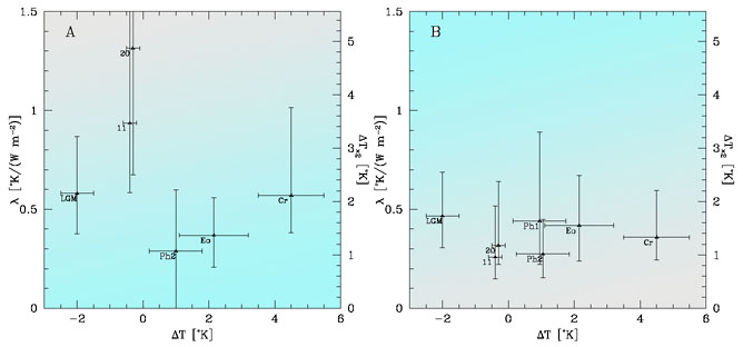
Figure 2 - The estimated sensitivity λ as a function of the average temperature ΔT relative to today over
which the sensitivity was calculated. The values are for the Last Glacial Maximum (LGM), 11 year solar cycle over the past 200 years (11), 20th century global warming (20), Phanerozoic
though comparison of the tropical temperature to CRF variations (Ph1) or to CO2 variations (Ph2), Eocene
(Eo) and Mid-Cretaceous (Cr). Panel (a) assumes that the CRF contributes no radiative forcing while panel
(b) assumes that the CRF does affect climate. Thus, the “Ph1” measurement is not applicable and does not
appear in panel (a). From the figures it is evident that: (i) The expectation value for λ is lower if CRF affects
climate. (ii) The values obtained using different paleoclimatic data are notably more consistent with each
other if CRF does affect climate (iii) There is no significant trend in λ vs. ΔT (there could have been if the ice/albedo feedback was large, as it operates only at low temperatures).
If the cosmic ray flux climate link is included in the radiation budget, averaging the different estimates for the sensitivity give a somewhat lower result, namely, that λ=0.35±0.09°K/(W m-2). (Corresponding to ΔTx2=1.3±0.4°). Interestingly, this result is quite similar to the so called "black body" (i.e., corresponding to a climate system with feedbacks that tend to cancel each other).
One of the most interesting points evident when comparing the two panels of fig. 2 is the fact that once the CRF is included in the sensitivity estimate, the scatter in the different sensitivity estimates is much smaller. This is strong empirical evidence suggesting that the CRF is indeed affecting the climate. The reason is that if the CRF would not have had any climatic effect, the CRF/climate corrections ΔSCRF would have corresponded to adding random numbers to the values on the left (i.e, to ΔS0, without the CRF). This would have tended to increase the scatter even more. However, once these "random" numbers were added, the scatter was significantly decreased instead, as you would expect if the corrections are real.
Summary
- Earth's climate sensitivity is not expected to be that of a "black body" because of different feedbacks known to exist in the climate system.
- Although Global Circulation models are excellent tools for studying some questions, they are very bad at predicting the global climate sensitivity because the cloud feedback is essentially unknown. It is the main reason why the sensitivity is (not) predicted this way with an uncertainty of a factor of 3!
- Climate Sensitivity can be estimated empirically. A relatively low value (one which corresponds to net cancelation of the feedbacks) is obtained.
- Empirical Climate sensitivities obtained on different time scales are significantly more consistent with each other if the Cosmic Ray flux / Climate link is included. This is yet another indication that this link is real.
Comments (5)
Thank you for posting this interesting blog.
Is there in your view any reason why the feedbacks cannot have a net negative value?
Hugh R
Dear Nir:
I enjoyed your article about estimation of climate sensitivity. However, you begin with an assertion that radiative forcing due to 2xCO2 is 3.8W/m2, all without any justification or explanation. I have some serious doubts in this estimation. The RealClimate website asserts that the article of Myhre at all (1998) is the most accurate estimate of radiative imbalance of Earth in case of man-made CO2 doubling. Myhre et al arrived at 3.7W/m2 of imbalance for 2xCO2. This is one of the critical baseline estimate used in the whole IPCC reporting and man-made global warming concept.
I wonder how did they do this? Obviously, the radiative cooling of warm gas is a relatively fast process - everybody knows that temperature can drop overnight to a substantial degree if skies are clear, so the process must be evaluated on at least 12-hour basis. We also all know that weather changes, and radiative conditions (clouds mostly) change sometimes on hourly basis. We all also know that cold areas sometimes have months of clear skies in winter (like in Siberia, where I was born and used to live for four decades). Obviously, given vast area of Siberia, Canada, mountain regions in central Asia, cooling by radiation to outer space must be important to global balance. How about all Arctic and Antarctic? We also know that the emitted radiation is strongly dependent on the vertical temperature shape of the atmospheric column in each particular place.
Yet, if we read the Myhre article of 1998. we find out the following startling revelation:
“Myhre and … have shown that for global radiative forcing calculations, it is not sufficient to use a single vertical profile”
It seems quite obvious to even a non-specialist in climate that Earth has more complex vertical profile of atmosphere than one tropical with clear skies. So, what is their scientific solution? They continue:
“ Freckelton at al [1998] have shown that three vertical profiles (a tropical profile and northern and southern hemisphere extratropical profiles) can represent global calculations sufficiently.”
So their best approach is three profiles, tropical and two “extratropical”. But where is Canada, Siberia, Mongolia? Where is the entire Antarctic continent? Where is North Pole? And what is the criteria for sufficient? Sufficient for what? [unfortunately I cannot find a copy of the Freckleton paper on web, but I doubt that their justification for only three profiles is satisfactory]
The other problem with these vertical “profiles” is that the typical scheme of radiative calculations uses so-called “adjusted profile” in accord with Hansen-IPCC recipe. The IPCC recipe is that after an instantaneous infusion of 2xCO2 the temperatures in stratosphere allegedly equilibrate first. So the process of stratospheric cooling seems to be excluded from calculations. Then it is assumed that the CO2 gets “well-mixed” rapidly, but the temperature near the radiative top of atmosphere remains unperturbed. As result, the CO2 emits from higher “colder” area, and thus causes the energy imbalance. This scheme has at least two substantial flaws with its physics.
First, the temperature in stratosphere increases with height, and this layer is usually assumed as stably stratified, and therefore does not have buoyant instability and corresponding mixing mechanisms. One would wonder how comes that a nearly motionless stable layer of air gets equilibrated much faster than the troposphere that is a subject of continuous convective stirring (which produces the proper polytropic lapse rate).
Second, it is well known in theory (and practice) of turbulence that passive scalars in turbulent media have nearly identical turbulent transport coefficients. Both temperature and CO2 are passive scalars, and therefore it is not physically possible to for CO2 to get mixed well ahead of temperature, they will mix simultaneously. This means that in practice the radiative forcing cannot exist at the level as it is proposed by IPCC-Hansen scheme, at least the imbalance must be much smaller.
Considering the above arguments, it is quite likely that the value of 3.8W/m2 is highly overestimated.
With kindest regards,
-Al Tekhasski
Hi Nir,
thanks a lot for this weblog -- I especially like the paper presented in this page.
* Have you heard about this paper from Dr. Gerhard Gerlich and Dr. Ralf D. Tscheuschner: http://arxiv.org/pdf/0707.1161 ?
To say it quickly, according to the authors, following what seems to me really serious physics (but I'm only a mechanical engineer) :
- the classical glass-house effect is mainly (let's say 95%) the consequence of an impossible convection inside the house, the radiative part of the problem being of really low effect (Wood's experimentation) ;
- there isn't nothing to call a greenhouse effect for the atmosphere / for gases. Scientif references are pretty rare, let's say circular, ... distorted (or even invented) by the IPCC itself and... completely wrong.
* Another paper, from Ferenc Miskolczi (he left the NASA in 2005 after the NASA refused to support this work) : http://met.hu/idojaras/IDOJARAS_vol111_No1_01.pdf
This study concludes that the atmospheric greenhouse effect is already saturated...
If ever you agree with (one of) those studies (if not, why ?) what would be the consequences on your study and results on climate sensitivity ?
Cheers.
I am a scientist, though not a climate scientist. For the past several years I have been trying to find climate papers on the internet, in order to seperate fact and fiction for myself. I had immediately, which is almost no one tries to explain their assertions and when they do there is always someone else saying why they're wrong.
The most frusterating part I encountered was climate sensitivity. This seemed to be the lynchpin to the whole global warming debate. Yet no one would explain climate sensitivity in all it's eccentricities. They would give a brief explaination (a doubling of CO2....) and tell me what the IPCC believes, but nothing more. How does the IPCC determine sensitivity? On what basis do others disagree? Why can't we (as the math seems to suggest) just look into the past and determine climate sensitivity without doubt? These questions remained unanswered- until you.
I am not naive enough to take what you say at face value. Nor do I believe that there isn't some guy out there who has an explaination for why everything you did was wrong. But I am appreciative that someone has finally stopped treating us like children and has given us solid details. Thank you.
Shaviv observed:
i.e. Shaviv finds a ratio of 2.9 times solar irradiance alone.
From initial data evaluation, Roy Spencer finds:
This supports Shaviv's results.
See: Indirect Solar Forcing of Climate by Galactic Cosmic Rays: An Observational Estimate